Asymptotic confidence intervals for NLS regression in R
Introduction
Nonlinear regression model
As a model setup, we consider noisy observations \(y_1,\ldots, y_n \in \mathbb{R}\) obtained from a standard nonlinear regression model of the form:
\[ \begin{aligned} y_i &\ = \ f(\boldsymbol{x}_i, \boldsymbol{\theta}) + \epsilon_i, \quad i = 1,\ldots, n \end{aligned} \] where \(f: \mathbb{R}^k \times \mathbb{R}^p \to \mathbb{R}\) is a known nonlinear function of the independent variables \(\boldsymbol{x}_1,\ldots,\boldsymbol{x}_n \in \mathbb{R}^k\) and the unknown parameter vector \(\boldsymbol{\theta} \in \mathbb{R}^p\) that we aim to estimate. The noise variables \(\epsilon_1, \ldots, \epsilon_n\) are assumed to be i.i.d. (not necessarily normally distributed) with \(\mathbb{E}[\epsilon_i] = 0\) and \(\text{Var}(\epsilon_i) = \sigma^2\).
Least squares estimation
In order to obtain a least squares estimate \(\hat{\boldsymbol{\theta}}\) of the parameter vector \(\boldsymbol{\theta}\), we minimize the error sum of squares according to:
\[ \hat{\boldsymbol{\theta}} \ = \ \arg \min_{\boldsymbol{\theta}} \sum_{i = 1}^n [y_i - f(\boldsymbol{x}_i, \boldsymbol{\theta})]^2 \]
Different optimization routines to minimize the above least squares criterion are available in base R (stats) or through a number of external R-packages and functions, see e.g. the Optimization and Mathematical Programming CRAN Task View for a comprehensive overview. In this post, we will focus on least-squares optimization using R’s default nls() function and the function nls.lm() from the minpack.lm-package, which performs least-squares optimization through a modification of the Levenberg-Marquadt algorithm.
Example 1: First-order reaction model
As a first example, let us generate \(n = 25\) noisy observations from a nonlinear first-order reaction model \(f: \mathbb{R} \times \mathbb{R}^2 \to \mathbb{R}\) of the form:
\[ f(x, \boldsymbol{\theta}) \ = \ \theta_1 \cdot (1 - \exp(-\exp(\theta_2) \cdot x)) \] with unknown parameter vector \(\boldsymbol{\theta} = (\theta_1, \theta_2)' \in \mathbb{R}^2\). Here, the parameter \(\theta_1\) can be interpreted as the horizontal asymptote (as \(x \to \infty\)) and \(\exp(\theta_2)\) corresponds to the rate constant in the reaction model.
The function values of \(f(x, \boldsymbol{\theta})\) (as well as its gradient) can be evaluated directly through the self-start model function SSasympOrig(). The true parameter values are set to \(\boldsymbol{\theta}^* = (\theta_1 = 1, \theta_2 = 1)'\) and the noise values \(\epsilon_1,\ldots,\epsilon_n\) are sampled from a normal distribution with mean zero and standard deviation \(\sigma = 0.05\).
library(ggplot2)

## parameters
n <- 25
sigma <- 0.05
theta <- c(Asym = 1, lrc = 1)

## simulate data
set.seed(1)
x1 <- (1:n) / n
f1 <- SSasympOrig(x1, Asym = theta["Asym"], lrc = theta["lrc"])
y1 <- rnorm(n, mean = f1, sd = sigma)

## plot data and expected response
ggplot(data = data.frame(x = x1, y = y1, f = f1), aes(x = x)) +
  geom_line(aes(y = f), lty = 2, color = "grey50") +
  geom_point(aes(y = y)) +
  theme_light() +
  labs(x = "Time (x)", y = "Response (y)", title = bquote("Simulated data" ~ list(y[1], ldots, y[n]) ~ "first-order reaction model" ~ list(theta[1] == 1, theta[2] == 1)))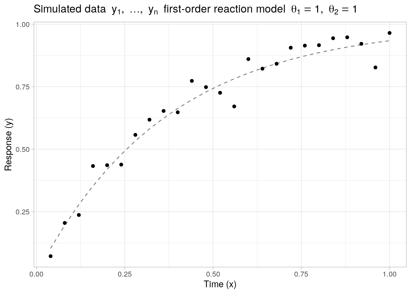
Given the noisy observations \(y_1,\ldots,y_n\), the least squares estimate \(\boldsymbol{\theta}\) is easily obtained with a call to nls() again using SSasympOrig() to specify the model formula:
## nls estimation with self-start model
nlsfit1 <- nls(
  y ~ SSasympOrig(x, Asym, lrc),
  data = data.frame(x = x1, y = y1)
)

summary(nlsfit1)
#>
#> Formula: y ~ SSasympOrig(x, Asym, lrc)
#>
#> Parameters:
#>      Estimate Std. Error t value Pr(>|t|)
#> Asym  1.00154    0.03325   30.12  < 2e-16 ***
#> lrc   1.03032    0.08378   12.30 1.35e-11 ***
#> ---
#> Signif. codes:  0 '***' 0.001 '**' 0.01 '*' 0.05 '.' 0.1 ' ' 1
#>
#> Residual standard error: 0.04825 on 23 degrees of freedom
#>
#> Number of iterations to convergence: 0
#> Achieved convergence tolerance: 5.287e-07
Example 2: Basic SIR model
As a second example, we look at a nonlinear model function \(f(x, \boldsymbol{\theta})\) with no simple closed-form expression, defined implicitly through a system of (ordinary) differential equations. Specifically, we consider \(f(x, \boldsymbol{\theta})\) to be the number of Infected individuals in a basic SIR model implicitly defined through the following set of differential equations1:
\[ \begin{aligned} \frac{dS(t)}{dt} & \ = \ - \frac{\beta I(t) S(t)}{N}, \\ \frac{dI(t)}{dt} & \ = \ \frac{\beta I(t) S(t)}{N} - \gamma I(t) \end{aligned} \] Using the same notation as before, the scalar independent variable \(x\) now corresponds to the time \(t\), and the nonlinear model function \(f(t, \boldsymbol{\theta})\) is given by \(I(t)\). The unknown parameters to estimate are \(\boldsymbol{\theta} = (\beta, \gamma)'\), and the initial conditions \(S(t_0)\) and \(I(t_0)\) are assumed to be given. Note that in this example \(f(x, \boldsymbol{\theta})\) is treated as a continuous function with as range the complete real line \(\mathbb{R}\), i.e. it is not restricted to only nonnegative integer values.
Below, we generate \(n = 50\) noisy observations \(y_1,\ldots,y_n\) based on a SIR model with true parameters \(\boldsymbol{\theta}^* = (\beta = 0.1, \gamma = 0.01)'\) and with errors sampled from a normal distribution with mean zero and standard deviation \(\sigma = 2.5\). The initial conditions are set to \(S(t_0) = 100\) and \(I(t_0) = 2\) and the times are evaluated at regular intervals across the time range \(t \in [10, 500]\).
library(deSolve)

## helper function to evaluate f(x, theta)
sir <- function(x, init, theta) {
  lsoda(
    y = init,
    times = x,
    func = function(t, y, parms, N) {
      with(as.list(parms), {
        list(c(
          S = -beta * y["I"] * y["S"] / N,
          I = beta * y["I"] * y["S"] / N - gamma * y["I"]
        ))
      })
    },
    parms = theta,
    N = sum(init)
  )[, "I"]
}

## parameters
n <- 50
sigma <- 2.5
theta <- c(beta = 0.1, gamma = 0.01)
init <- c(S = 100, I = 2)

## simulated data
set.seed(1)
x2 <- 10 * (1:n)
f2 <- sir(x2, init, theta)
y2 <- rnorm(n, mean = f2, sd = sigma)

## plot data and expected response
ggplot(data = data.frame(x = x2, y = y2, f = f2), aes(x = x)) +
  geom_line(aes(y = f), lty = 2, color = "grey50") +
  geom_point(aes(y = y)) +
  theme_light() +
  labs(x = "Time (x)", y = "Response (y)", title = bquote("Simulated data" ~ list(y[1], ldots, y[n]) ~ "infected compartment SIR model" ~ list(beta == 0.1, gamma == 0.01)))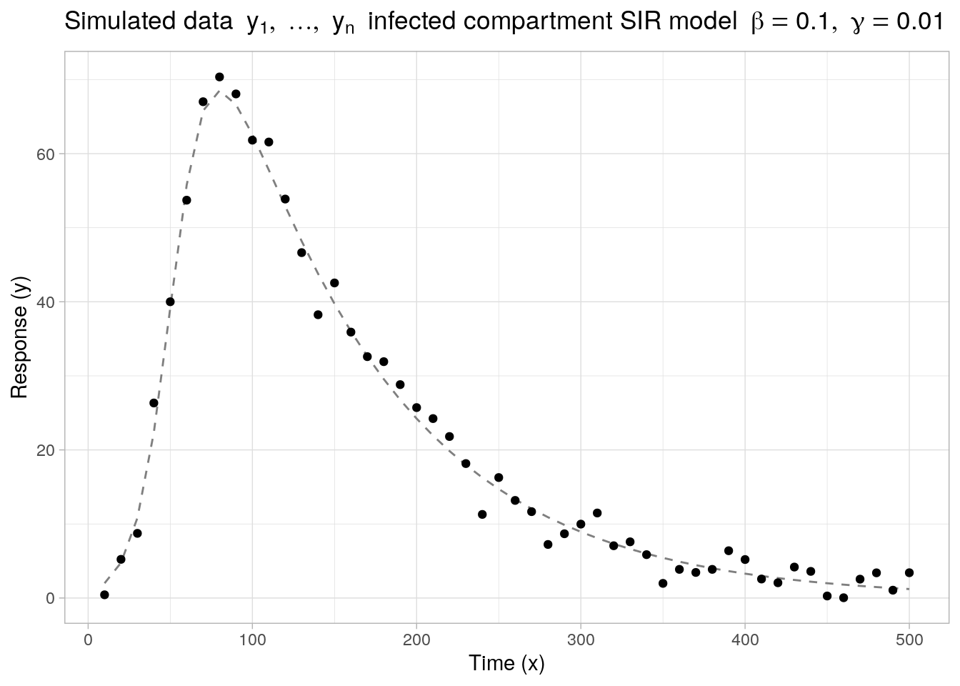
Instead of using the nls() function to obtain the least squares estimate \(\hat{\boldsymbol{\theta}}\), we minimize the error sum of squares by means of the Levenberg-Marquadt algorithm with a call to minpack.lm::nls.lm()2. The nls.lm() function requires as input a function fn evaluating to the vector of residuals \(\{y_i - f(x_i, \boldsymbol{\theta}) \}_{i=1}^n\) for a given parameter vector \(\boldsymbol{\theta}\):
library(minpack.lm)

nlsfit2 <- nls.lm(
  fn = function(par, data, init) {
    data[["y"]] - sir(data[["x"]], init, par) ## residuals
  },
  par = c(beta = 0, gamma = 0),               ## starting values
  data = data.frame(x = x2, y = y2),          ## observations
  init = init                                 ## fixed values
)

summary(nlsfit2)
#>
#> Parameters:
#>       Estimate Std. Error t value Pr(>|t|)
#> beta  0.100549   0.001335   75.33   <2e-16 ***
#> gamma 0.009877   0.000135   73.15   <2e-16 ***
#> ---
#> Signif. codes:  0 '***' 0.001 '**' 0.01 '*' 0.05 '.' 0.1 ' ' 1
#>
#> Residual standard error: 2.097 on 48 degrees of freedom
#> Number of iterations to termination: 13
#> Reason for termination: Relative error in the sum of squares is at most `ftol'.
Asymptotic confidence intervals for parameters
Theory
For sufficiently large \(n\), and subject to appropriate regularity assumptions, (such as \(f(\boldsymbol{x}, \boldsymbol{\theta})\) being twice continuously differentiable with respect to \(\boldsymbol{\theta}\)), the least squares estimate \(\hat{\boldsymbol{\theta}}\) is approximately normally distributed according to3:
\[ \hat{\boldsymbol{\theta}} \ \overset{\cdot}{\sim} \ N_p(\boldsymbol{\theta}^*, \sigma^2\left(\boldsymbol{F}_\cdot(\boldsymbol{\theta}^*)'\boldsymbol{F}_\cdot(\boldsymbol{\theta}^*) \right)^{-1}) \] Here, \(\boldsymbol{\theta}^*\) is the true value of \(\boldsymbol{\theta}\), and
\[ \boldsymbol{F}_{\cdot}(\boldsymbol{\theta}^*) \ = \ \left[ \dfrac{\partial f(\boldsymbol{x}_i, \boldsymbol{\theta})}{\partial \theta_j}\Bigg|_{\boldsymbol{\theta} = \boldsymbol{\theta}^*} \right]_{i,j} \in \mathbb{R}^{n \times p} \]
is the matrix of gradient vectors of \(f(\boldsymbol{x}, \boldsymbol{\theta})\) evaluated at \(\boldsymbol{\theta} = \boldsymbol{\theta}^*\), with the \(i\)-th row of the matrix corresponding to (the transpose of) the gradient vector \(\nabla f(\boldsymbol{x}_i, \boldsymbol{\theta}) \in \mathbb{R}^p\) evaluated at \(\boldsymbol{\theta}^*\).
Replacing \(\sigma^2\) by the variance estimate \(s^2 = \sum_{i = 1}^n (y_i - f(\boldsymbol{x}_i, \hat{\boldsymbol{\theta}}))^2 / (n - p)\), an approximate \(100(1 - \alpha)\%\) joint confidence region for \(\boldsymbol{\theta}^*\) can be constructed by the ellipsoid:
\[ \big\{ \boldsymbol{\theta} \ : \ (\boldsymbol{\theta} - \hat{\boldsymbol{\theta}})'\boldsymbol{F}_\cdot(\hat{\boldsymbol{\theta}})'\boldsymbol{F}_\cdot(\hat{\boldsymbol{\theta}})(\boldsymbol{\theta} - \hat{\boldsymbol{\theta}}) \leq p s^2 F^{p, n-p}_{1-\alpha} \} \] where \(F^{p, n-p}_{1-\alpha}\) denotes the \(1-\alpha\) quantile of an F-distribution with \(p\) and \(n-p\) degrees of freedom.
Also, approximate \(100(1 - \alpha)\%\) marginal confidence intervals for the individual parameters are given by:
\[ \Big[ \hat{\theta}_\ell - s \sqrt{\big(\boldsymbol{F}_\cdot(\hat{\boldsymbol{\theta}})'\boldsymbol{F}_\cdot(\hat{\boldsymbol{\theta}})\big)^{-1}_{\ell\ell}} t_{1 - \alpha/2}^{n - p}, \hat{\theta}_\ell + s \sqrt{\big(\boldsymbol{F}_\cdot(\hat{\boldsymbol{\theta}})'\boldsymbol{F}_\cdot(\hat{\boldsymbol{\theta}})\big)^{-1}_{\ell\ell}} t_{1 - \alpha/2}^{n - p} \Big], \quad \text{for}\ \ell = 1,\ldots, n \] with \(\big(\boldsymbol{F}_\cdot(\hat{\boldsymbol{\theta}})'\boldsymbol{F}_\cdot(\hat{\boldsymbol{\theta}})\big)^{-1}_{\ell\ell}\) the \(\ell\)-th diagonal term of \(\big(\boldsymbol{F}_\cdot(\hat{\boldsymbol{\theta}})'\boldsymbol{F}_\cdot(\hat{\boldsymbol{\theta}})\big)^{-1}\), and \(t^{n-p}_{1 - \alpha/2}\) the \(1 - \alpha/2\) quantile of a t-distribution with \(n - p\) degrees of freedom.
The above asymptotic results rely on a linear approximation of \(f(\boldsymbol{x}, \boldsymbol{\theta})\) in a small neighborhood of \(\boldsymbol{\theta}^*\) in combination with the application of an appropriate central limit theorem (in the context of a linear regression problem). Rigorous proofs can be found in a number of textbooks, for instance (Seber and Wild 2003, Chapters 2 and 12) or (Amemiya 1985, Chapter 4).
Remark
If \(f(\boldsymbol{x}_i, \boldsymbol{\theta})\) with \(\boldsymbol{x}_i, \boldsymbol{\theta} \in \mathbb{R}^p\) is a linear function of \(\boldsymbol{\theta}\), i.e. \[ f(\boldsymbol{x}_i, \boldsymbol{\theta}) \ = \ \boldsymbol{x}_i' \boldsymbol{\theta} \ = \ x_{i1}\theta_1 + \ldots + x_{ip}\theta_p, \]
then the gradient matrix \(\boldsymbol{F}_{\cdot}(\boldsymbol{\theta})\) is independent of \(\boldsymbol{\theta}\) and reduces to the design matrix \(\boldsymbol{F}_{\cdot}(\boldsymbol{\theta}) = \boldsymbol{X} \in \mathbb{R}^{n \times p}\) with the \(i\)-th row of \(\boldsymbol{X}\) corresponding to \(\boldsymbol{x}_i\). Substituting \(\boldsymbol{F}_{\cdot}(\hat{\boldsymbol{\theta}}) = \boldsymbol{X}\) in the above expressions, we obtain the usual asymptotic results for (ordinary) least squares estimation in a multiple linear regression context, see also (Seber and Wild 2003, Appendix D) or (Bates and Watts 1988, Chapter 1).
Application
Based on the listed asymptotic results, we evaluate marginal (asymptotic) parameter confidence intervals centered around the least squares estimates \(\hat{\boldsymbol{\theta}}\) obtained for the example models in the previous section. Where possible we compare the manual calculations to standard methods available for objects of class nls and nls.lm respectively.
Example 1 (continued)
First, to evaluate the gradient matrix \(\boldsymbol{F}_\cdot(\hat{\boldsymbol{\theta}})\) in the context of the first-order reaction model example, we can make use of the deriv() function, which calculates exact (symbolic) derivatives for a number of common mathematical functions and compositions thereof. The deriv() function returns an expression, which we evaluate at the given inputs \(x_1,\ldots,x_n\) and least squares estimates \(\hat{\boldsymbol{\theta}}\).
## symbolic derivative f(x, theta)
(dtheta <- deriv(~ Asym * (1 - exp(-exp(lrc) * x)), c("Asym", "lrc")))
#> expression({
#>     .expr1 <- exp(lrc)
#>     .expr4 <- exp(-.expr1 * x)
#>     .expr5 <- 1 - .expr4
#>     .value <- Asym * .expr5
#>     .grad <- array(0, c(length(.value), 2L), list(NULL, c("Asym",
#>         "lrc")))
#>     .grad[, "Asym"] <- .expr5
#>     .grad[, "lrc"] <- Asym * (.expr4 * (.expr1 * x))
#>     attr(.value, "gradient") <- .grad
#>     .value
#> })
## least squares estimates
cc <- coef(nlsfit1)
## gradient matrix
(Fdot <- attr(eval(dtheta, envir = list(x = x1, Asym = cc["Asym"], lrc = cc["lrc"])), "gradient"))
#> Asym lrc
#> [1,] 0.1060259 0.1003495
#> [2,] 0.2008104 0.1794197
#> [3,] 0.2855452 0.2405949
#> [4,] 0.3612959 0.2867808
#> [5,] 0.4290151 0.3204682
#> [6,] 0.4895543 0.3437883
#> [7,] 0.5436748 0.3585608
#> [8,] 0.5920571 0.3663361
#> [9,] 0.6353096 0.3684319
....The same gradient matrix can also directly be extracted from the the nls object itself:
## existing gradient matrix
Fdot1 <- nlsfit1$m$gradient()
all.equal(Fdot, Fdot1)
#> [1] TRUE
Fdotfit1 <- Fdot ## save for later useSecond, we compute the estimate \(s\) for the residual standard deviation \(\sigma\), which can either be done manually or using the sigma() method for objects of class nls:
## residual standard deviation
s <- sqrt(sum(residuals(nlsfit1)^2) / df.residual(nlsfit1))
s1 <- sigma(nlsfit1)
all.equal(s, s1)
#> [1] TRUE
The estimated (asymptotic) covariance matrix of \(\hat{\boldsymbol{\theta}}\) then follows from \(s^2\left(\boldsymbol{F}_\cdot(\hat{\boldsymbol{\theta}})'\boldsymbol{F}_\cdot(\hat{\boldsymbol{\theta}})\right)^{-1}\):
## asymptotic covariance matrix
Sigma <- s^2 * solve(t(Fdot) %*% Fdot)
Sigma1 <- vcov(nlsfit1)
all.equal(Sigma, Sigma1)
#> [1] TRUE
And the marginal parameter confidence intervals are calculated as usual by scaling the quantiles of a t-distribution with the standard errors obtained from the diagonal of the estimated (asymptotic) covariance matrix:
## asymptotic ci's
cc + sqrt(diag(Sigma)) %o% qt(c(0.025, 0.975), df.residual(nlsfit1))
#>           [,1]     [,2]
#> Asym 0.9327486 1.070330
#> lrc  0.8570054 1.203635
The same confidence intervals can also be obtained directly with nlstools::confint2()by setting method = "asysmptotic":
nlstools::confint2(nlsfit1, level = 0.95, method = "asymptotic")
#>          2.5 %   97.5 %
#> Asym 0.9327486 1.070330
#> lrc  0.8570054 1.203635
Remark
Inside the nls() function, the inverse \((\boldsymbol{F}_\cdot(\hat{\boldsymbol{\theta}})'\boldsymbol{F}_\cdot(\hat{\boldsymbol{\theta}}))^{-1}\) is evaluated by means of a QR decomposion of \(\boldsymbol{F}_\cdot(\hat{\boldsymbol{\theta}})\), i.e. \(\boldsymbol{F}_\cdot(\hat{\boldsymbol{\theta}}) = \boldsymbol{Q}\boldsymbol{R}\) with orthogonal matrix \(\boldsymbol{Q}' = \boldsymbol{Q}^{-1}\) and \(\boldsymbol{R}\) an upper triangular matrix. The inverse of the matrix product then relies only on the upper triangular matrix \(\boldsymbol{R}\), since:
\[ (\boldsymbol{F}_\cdot(\hat{\boldsymbol{\theta}})'\boldsymbol{F}_\cdot(\hat{\boldsymbol{\theta}}))^{-1} = (\boldsymbol{R}'\boldsymbol{Q}'\boldsymbol{Q}\boldsymbol{R})^{-1} = (\boldsymbol{R}'\boldsymbol{Q}^{-1}\boldsymbol{Q}\boldsymbol{R})^{-1} = (\boldsymbol{R}'\boldsymbol{R})^{-1} \]
and the expression on the right-hand side can be evaluated efficiently through R’s chol2inv() function.
## cholesky-based evaluation
Sigma2 <- s^2 * chol2inv(qr.R(qr(Fdot)))
all.equal(unname(Sigma), Sigma2)
#> [1] TRUE
Example 2 (continued)
For the basic SIR-model, no simple closed-form expression of \(f(x, \boldsymbol{\theta})\) is available, thus we can no longer use the deriv() function for exact differentiation of the model function \(f\). Instead, we approximate the gradient numerically through finite differencing with the numericDeriv() function:
## least squares estimates
cc <- nlsfit2$par

## numeric approximation gradient matrix
rho <- list2env(list(x = x2, init = init, beta = cc["beta"], gamma = cc["gamma"]))
expr <- quote(sir(x, init, theta = c(beta, gamma)))
(Fdot <- attr(numericDeriv(expr, theta = c("beta", "gamma"), rho), "gradient"))
#>              [,1]        [,2]
#>  [1,]    0.000000     0.00000
#>  [2,]   45.496517   -47.68031
#>  [3,]  192.589702  -212.32052
#>  [4,]  504.949233  -613.32713
#>  [5,]  846.769842 -1238.81362
#>  [6,]  868.528689 -1797.93112
#>  [7,]  558.561159 -2123.23154
#>  [8,]  214.999332 -2344.13588
#>  [9,]  -13.914997 -2567.05553
....
Fdotfit2 <- Fdot ## save for later useThe estimated residual standard deviation \(s\) and asymptotic covariance matrix are computed the same way as before:
## residual standard deviation
s <- sqrt(sum((y2 - sir(x2, init, cc))^2) / (length(y2) - length(cc)))
s1 <- sqrt(nlsfit2$deviance / (df.residual(nlsfit2)))
all.equal(s, s1)
#> [1] TRUE

## asymptotic covariance matrix
(Sigma <- s^2 * solve(t(Fdot) %*% Fdot))
#>               [,1]          [,2]
#> [1,]  1.781511e-06 -3.311626e-08
#> [2,] -3.311626e-08  1.823114e-08
(Sigma1 <- vcov(nlsfit2))
#>                beta         gamma
#> beta   1.781513e-06 -3.311644e-08
#> gamma -3.311644e-08  1.823147e-08
As well as the marginal parameter confidence intervals:
## asymptotic ci's
cc + sqrt(diag(Sigma)) %o% qt(c(0.025, 0.975), df.residual(nlsfit2))
#>            [,1]       [,2]
#> [1,] 0.09786537 0.10323269
#> [2,] 0.00960596 0.01014892
The manually calculated confidence intervals are slightly wider than the asymptotic confidence intervals returned by the confint() method of an object of class nls.lm. This is because the latter uses quantiles from a normal distribution instead of a t-distribution:
confint(nlsfit2, level = 0.95) ## normal quantiles
#>             2.5 %     97.5 %
#> beta  0.097933001 0.10316506
#> gamma 0.009612799 0.01014208
Asymptotic confidence intervals for expected response
Theory
Besides inference with respect to the model parameters, we are often also interested in inference with respect to the nonlinear model function \(f(\boldsymbol{x}, \boldsymbol{\theta})\). Subject to the same regularity assumptions as in the previous section, starting from the asymptotic normality of the least squares estimate:
\[ \hat{\boldsymbol{\theta}} \ \overset{\cdot}{\sim} \ N_p(\boldsymbol{\theta}^*, \sigma^2\left(\boldsymbol{F}_\cdot(\boldsymbol{\theta}^*)'\boldsymbol{F}_\cdot(\boldsymbol{\theta}^*) \right)^{-1}) \]
Asymptotic normality of \(f(\boldsymbol{x}_i, \hat{\boldsymbol{\theta}})\) or some other function \(g \in \mathcal{C}^1\) of \(\boldsymbol{\theta}\) follows by an application of the (multivariate) delta method, such that for sufficiently large \(n\):
\[ f(\boldsymbol{x}_i, \hat{\boldsymbol{\theta}}) \ \overset{\cdot}{\sim} \ N(f(\boldsymbol{x}_i, \boldsymbol{\theta}^*)), \sigma^2 \nabla f(\boldsymbol{x}_i, \boldsymbol{\theta}^*)' \left(\boldsymbol{F}_\cdot(\boldsymbol{\theta}^*)'\boldsymbol{F}_\cdot(\boldsymbol{\theta}^*)\right)^{-1}\nabla f(\boldsymbol{x}_i, \boldsymbol{\theta}^*)) \]
where \(\nabla f(\boldsymbol{x}_i, \boldsymbol{\theta}^*) \in \mathbb{R}^{p}\) is the gradient vector of \(f(\boldsymbol{x}_i, \boldsymbol{\theta})\) evaluated at \(\boldsymbol{\theta}^*\), which corresponds to the (transpose of the) \(i\)-th row of \(\boldsymbol{F}_{\cdot}(\boldsymbol{\theta}^*)\).
Replacing \(\sigma^2\) by the same variance estimate as before, \(s^2 = \sum_{i = 1}^n (y_i - f(\boldsymbol{x}_i, \hat{\boldsymbol{\theta}}))^2 / (n - p)\), and evaluating the gradients at \(\hat{\boldsymbol{\theta}}\) instead of \(\boldsymbol{\theta}^*\), approximate \(100(1 - \alpha)\%\) confidence intervals for \(f(\boldsymbol{x}_i, \boldsymbol{\theta})\) are constructed as:
\[ f(\boldsymbol{x}_i, \hat{\boldsymbol{\theta}}) \pm s \sqrt{\nabla f(\boldsymbol{x}_i, \hat{\boldsymbol{\theta}})' \left(\boldsymbol{F}_\cdot(\hat{\boldsymbol{\theta}})'\boldsymbol{F}_\cdot(\hat{\boldsymbol{\theta}})\right)^{-1}\nabla f(\boldsymbol{x}_i, \hat{\boldsymbol{\theta}})} t^{n - p}_{1 - \alpha / 2} \]
In order to construct an approximate prediction interval for the response \(y_i\), we only need to rescale the above standard errors to include an additional variance term \(\text{Var}(\epsilon_i) = \sigma^2\), which follows heuristically by decomposing \(\text{Var}(y_i - f(\boldsymbol{x}_i, \hat{\boldsymbol{\theta}}))\) according to:
\[ \begin{aligned} \text{Var}(y_i - f(\boldsymbol{x}_i, \hat{\boldsymbol{\theta}})) & \ \approx \ \text{Var}(y_i) + \text{Var}(f(\boldsymbol{x}_i, \hat{\boldsymbol{\theta}})) \\ & \ \approx \ \sigma^2 + \sigma^2 \nabla f(\boldsymbol{x}_i, \boldsymbol{\theta}^*)' \left(\boldsymbol{F}_\cdot(\boldsymbol{\theta}^*)'\boldsymbol{F}_\cdot(\boldsymbol{\theta}^*)\right)^{-1}\nabla f(\boldsymbol{x}_i, \boldsymbol{\theta}^*) \end{aligned} \] The first step relies on the asymptotic independence of \(\epsilon_i\) and \(\hat{\boldsymbol{\theta}}\) (see (Seber and Wild 2003, Ch. 2)), and the second step follows by plugging in the asymptotic variance of \(f(\boldsymbol{x}_i, \hat{\boldsymbol{\theta}})\) obtained via the delta method above. For a more detailed description, see (Seber and Wild 2003, Ch. 5).
By substituting \(s^2\) for \(\sigma^2\) and evaluating the gradients at the least squares estimate \(\hat{\boldsymbol{\theta}}\), approximate \(100(1 - \alpha)\%\) prediction intervals for the individual response \(y_i\) can be constructed as:
\[ f(\boldsymbol{x}_i, \hat{\boldsymbol{\theta}}) \pm s \sqrt{1 + \nabla f(\boldsymbol{x}_i, \hat{\boldsymbol{\theta}})' \left(\boldsymbol{F}_\cdot(\hat{\boldsymbol{\theta}})'\boldsymbol{F}_\cdot(\hat{\boldsymbol{\theta}})\right)^{-1}\nabla f(\boldsymbol{x}_i, \hat{\boldsymbol{\theta}})} t^{n - p}_{1 - \alpha / 2} \]
Remark
Note that if we again consider a linear model function \(f(\boldsymbol{x}_i, \boldsymbol{\theta}) = \boldsymbol{x}_i'\boldsymbol{\theta}\) with \(\boldsymbol{x}_i, \boldsymbol{\theta} \in \mathbb{R}^p\), then the confidence intervals for the expected response reduce to:
\[ \boldsymbol{x}_i'\hat{\boldsymbol{\theta}} \pm s \sqrt{\boldsymbol{x}_i'(\boldsymbol{X}'\boldsymbol{X})^{-1}\boldsymbol{x}_i} t^{n-p}_{1 - \alpha/2} \] which corresponds to the standard asymptotic results for ordinary least squares estimation in a multiple linear regression context, see (Bates and Watts 1988, Chapter 1).
Application
We evaluate the approximate confidence intervals for the expected responses, as well as the approximate prediction intervals for the individual responses, based on the least squares estimates \(\hat{\boldsymbol{\theta}}\) obtained for the example models above. The gradients necessary to construct the confidence and prediction intervals can be recycled directly from the previous section, we only need to combine the available terms according to the above expressions.
Example 1 (continued)
Confidence intervals for the expected response
## asymptotic ci's expected response
fit <- fitted(nlsfit1)
Fdot <- Fdotfit1
ses <- sigma(nlsfit1) * sqrt(rowSums(Fdot %*% solve(t(Fdot) %*% Fdot) * Fdot))

ci <- fit + ses %o% qt(c(0.025, 0.975), df.residual(nlsfit1))
cimat <- cbind(fit = fit, lwr = ci[, 1], upr = ci[, 2])
The same approximate confidence intervals (for objects of class nls) can be generated using e.g. the predFit() method available through the investr-package:
cimat1 <- investr::predFit(nlsfit1, interval = "confidence", level = 0.95)
all.equal(cimat, cimat1)
#> [1] TRUE
## plot least squares fitted response and ci's
ggplot(data = cbind(data.frame(x = x1, f = f1), cimat), aes(x = x)) +
geom_ribbon(aes(ymin = lwr, ymax = upr), color = "grey70", alpha = 0.25, fill = "grey50") +
geom_line(aes(y = f), lty = 2) +
geom_line(aes(y = fit)) +
theme_light() +
labs(x = "Time (x)", y = "Response (y)", subtitle = "First-order reaction model",
title = "Approximate 95%-confidence intervals expected response")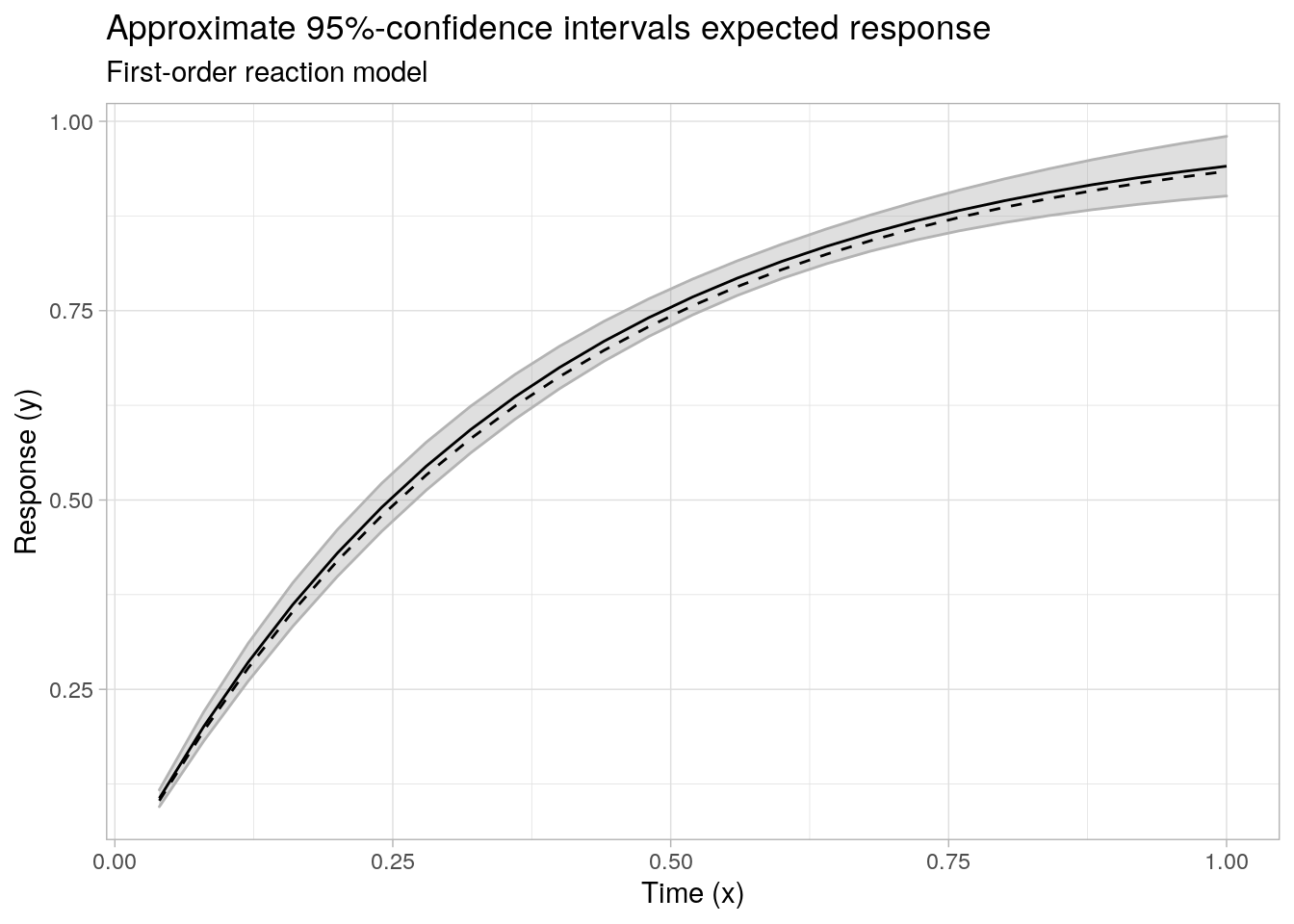
Prediction intervals for the responses
## asymptotic pi's individual reponses
ses <- sigma(nlsfit1) * sqrt(1 + rowSums(Fdot %*% solve(t(Fdot) %*% Fdot) * Fdot))

pi <- fit + ses %o% qt(c(0.025, 0.975), df.residual(nlsfit1))
(pimat <- cbind(fit = fit, lwr = pi[, 1], upr = pi[, 2]))
#>             fit         lwr       upr
#>  [1,] 0.1061891 0.005761992 0.2066163
#>  [2,] 0.2011195 0.099468204 0.3027707
#>  [3,] 0.2859847 0.183096588 0.3888729
#>  [4,] 0.3618521 0.257993080 0.4657111
#>  [5,] 0.4296755 0.325203806 0.5341472
#>  [6,] 0.4903079 0.385572691 0.5950431
#>  [7,] 0.5445117 0.439803826 0.6492196
#>  [8,] 0.5929685 0.488501007 0.6974359
#>  [9,] 0.6362876 0.532193231 0.7403819
....
pimat1 <- investr::predFit(nlsfit1, interval = "prediction", level = 0.95)
all.equal(pimat, pimat1)
#> [1] TRUE## plot least squares fitted response and pi's
ggplot(data = cbind(data.frame(x = x1, y = y1), pimat), aes(x = x)) +
geom_ribbon(aes(ymin = lwr, ymax = upr), color = "grey70", alpha = 0.25, fill = "grey50") +
geom_point(aes(y = y)) +
geom_line(aes(y = fit), color = "black") +
theme_light() +
labs(x = "Time (x)", y = "Response (y)", subtitle = "First-order reaction model",
title = "Approximate 95%-prediction intervals individual responses")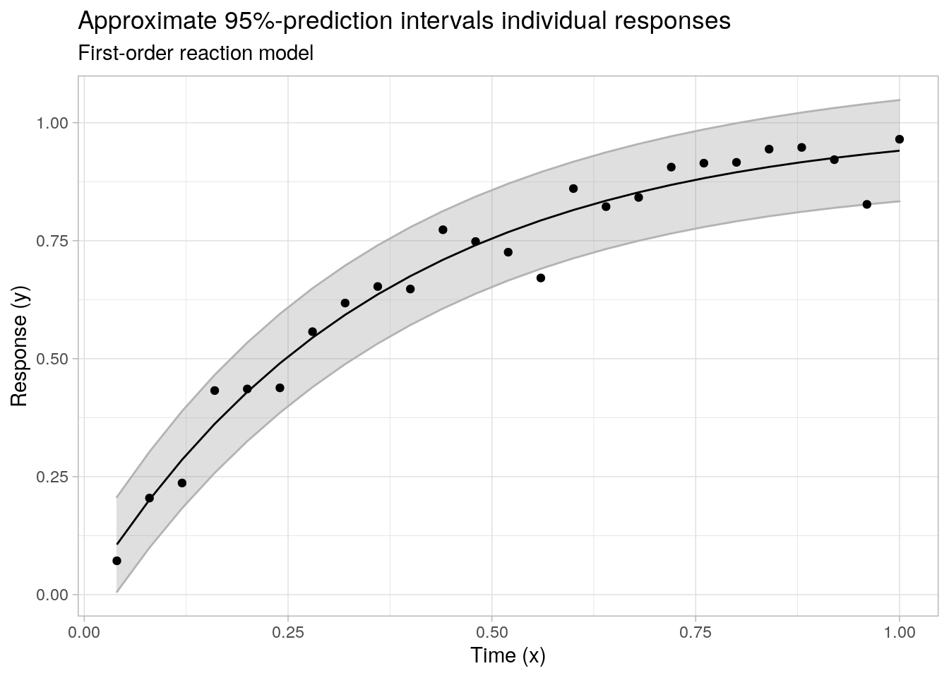
Example 2 (continued)
For the SIR model fit, we recycle the gradient matrix obtained through numerical differentiation of \(f(\boldsymbol{x}_i, \boldsymbol{\theta})\). Note that the investr::predFit() method can no longer be used to construct the same confidence and prediction intervals as no implementation is available for objects of class nls.lm.
Confidence intervals for the expected response
## asymptotic ci's expected response
cc <- nlsfit2$par
fit <- sir(x2, init = init, theta = cc)
Fdot <- Fdotfit2
s <- sqrt(nlsfit2$deviance / df.residual(nlsfit2))
ses <-  s * sqrt(rowSums(Fdot %*% solve(t(Fdot) %*% Fdot) * Fdot))

ci <- fit + ses %o% qt(c(0.025, 0.975), df.residual(nlsfit2))
(cimat <- cbind(fit = fit, lwr = ci[, 1], upr = ci[, 2]))
#>             fit       lwr       upr
#>  [1,]  2.000000  2.000000  2.000000
#>  [2,]  4.792016  4.666892  4.917141
#>  [3,] 10.951896 10.421425 11.482368
#>  [4,] 22.696320 21.300979 24.091661
#>  [5,] 39.795790 37.438255 42.153326
#>  [6,] 56.469689 54.002068 58.937310
#>  [7,] 66.366614 64.664624 68.068603
#>  [8,] 68.922863 67.988599 69.857126
#>  [9,] 66.933463 66.242441 67.624485
....
## plot least squares fitted response and ci's
ggplot(data = cbind(data.frame(x = x2, f = f2), cimat), aes(x = x)) +
geom_ribbon(aes(ymin = lwr, ymax = upr), color = "grey70", alpha = 0.25, fill = "grey50") +
geom_line(aes(y = f), lty = 2) +
geom_line(aes(y = fit), color = "black") +
theme_light() +
labs(x = "Time (x)", y = "Response (y)", subtitle = "Infected compartment SIR model",
title = "Approximate 95%-confidence intervals expected response")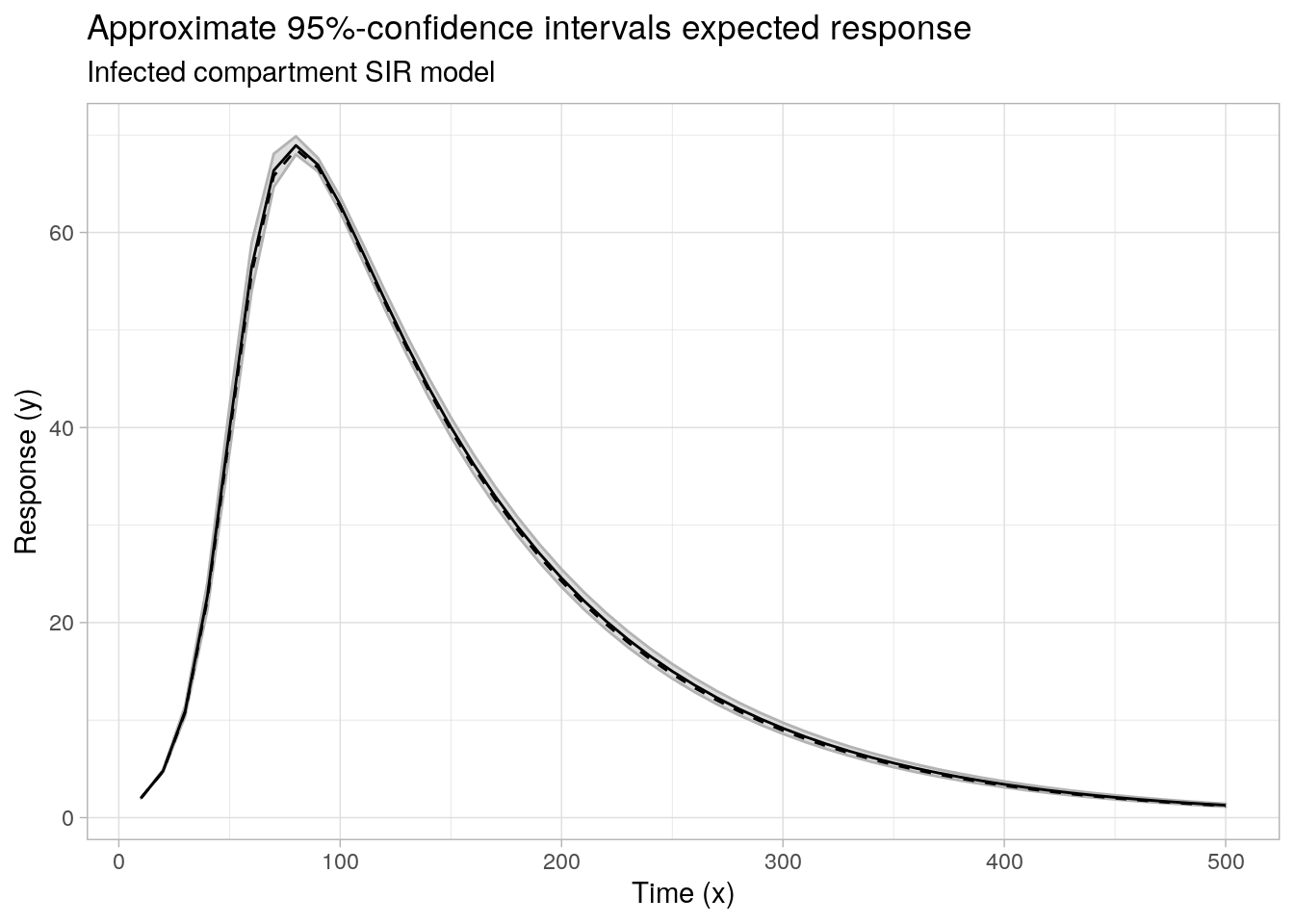
Prediction intervals for the responses
## asymptotic pi's individual reponses
ses <- s * sqrt(1 + rowSums(Fdot %*% solve(t(Fdot) %*% Fdot) * Fdot))

pi <- fit + ses %o% qt(c(0.025, 0.975), df.residual(nlsfit1))
(pimat <- cbind(fit = fit, lwr = pi[, 1], upr = pi[, 2]))
#>             fit        lwr       upr
#>  [1,]  2.000000 -2.3371178  6.337118
#>  [2,]  4.792016  0.4529884  9.131044
#>  [3,] 10.951896  6.5805732 15.323220
#>  [4,] 22.696320 18.1277796 27.264860
#>  [5,] 39.795790 34.8264871 44.765094
#>  [6,] 56.469689 51.4441284 61.495249
#>  [7,] 66.366614 61.6893323 71.043895
#>  [8,] 68.922863 64.4805047 73.365220
#>  [9,] 66.933463 62.5384591 71.328467
....
## plot least squares fitted response and pi's
ggplot(data = cbind(data.frame(x = x2, y = y2), pimat), aes(x = x)) +
geom_ribbon(aes(ymin = lwr, ymax = upr), color = "grey70", alpha = 0.25, fill = "grey50") +
geom_point(aes(y = y)) +
geom_line(aes(y = fit)) +
theme_light() +
labs(x = "Time (x)", y = "Response (y)", subtitle = "Infected compartment SIR model",
title = "Approximate 95%-prediction intervals individual responses")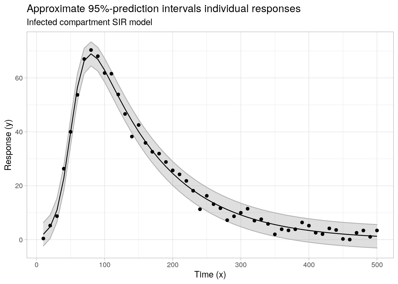
Session Info
sessionInfo()
#> R version 4.0.2 (2020-06-22)
#> Platform: x86_64-pc-linux-gnu (64-bit)
#> Running under: Ubuntu 18.04.5 LTS
#>
#> Matrix products: default
#> BLAS:   /usr/lib/x86_64-linux-gnu/blas/libblas.so.3.7.1
#> LAPACK: /usr/lib/x86_64-linux-gnu/lapack/liblapack.so.3.7.1
#>
#> locale:
#>  [1] LC_CTYPE=en_US.UTF-8       LC_NUMERIC=C
#>  [3] LC_TIME=en_US.UTF-8        LC_COLLATE=en_US.UTF-8
#>  [5] LC_MONETARY=en_US.UTF-8    LC_MESSAGES=en_US.UTF-8
#>  [7] LC_PAPER=en_US.UTF-8       LC_NAME=C
#>  [9] LC_ADDRESS=C               LC_TELEPHONE=C
#> [11] LC_MEASUREMENT=en_US.UTF-8 LC_IDENTIFICATION=C
#>
#> attached base packages:
#> [1] stats     graphics  grDevices utils     datasets  methods   base
#>
#> other attached packages:
#> [1] minpack.lm_1.2-1 deSolve_1.28     ggplot2_3.3.3
#>
#> loaded via a namespace (and not attached):
#>  [1] investr_1.4.0     highr_0.8         bslib_0.2.4       compiler_4.0.2
#>  [5] pillar_1.4.7      jquerylib_0.1.3   nlstools_1.0-2    tools_4.0.2
#>  [9] digest_0.6.27     lattice_0.20-41   nlme_3.1-149      jsonlite_1.7.2
#> [13] evaluate_0.14     lifecycle_0.2.0   tibble_3.0.6      gtable_0.3.0
#> [17] pkgconfig_2.0.3   rlang_0.4.10      DBI_1.1.1         yaml_2.2.1
#> [21] blogdown_1.2      xfun_0.22         withr_2.4.1       stringr_1.4.0
#> [25] dplyr_1.0.4       knitr_1.31        generics_0.1.0    sass_0.3.1
#> [29] vctrs_0.3.6       grid_4.0.2        tidyselect_1.1.0  glue_1.4.2
#> [33] R6_2.5.0          rmarkdown_2.6.6   bookdown_0.21     farver_2.0.3
#> [37] purrr_0.3.4       magrittr_2.0.1    scales_1.1.1      htmltools_0.5.1.1
#> [41] ellipsis_0.3.1    assertthat_0.2.1  colorspace_2.0-0  labeling_0.4.2
#> [45] stringi_1.5.3     munsell_0.5.0     crayon_1.4.1
References
Amemiya, T. 1985. Advanced Econometrics.
Bates, D. M., and D. G. Watts. 1988. Nonlinear Regression Analysis and Its Applications.
Seber, G. A. F., and C. J. Wild. 2003. Nonlinear Regression.